
In the previous chapter, you learned the core building blocks of an LLM application with LangChain and built a simple chatbot that sends a prompt to a model and returns its response. While useful, this setup has important limitations.
What happens when your use case depends on information the model wasn’t trained on? For example, asking questions about a company using data stored in a private PDF. Even though model providers continually expand their training data with public information, two key gaps remain:
- Private data: Information that isn’t publicly available is not included in LLM training.
- Current events: Because training is expensive and slow, models have a knowledge cutoff and lack awareness of events after their training data was finalized.
In both cases, the model is likely to hallucinate and return inaccurate answers. Prompt tweaks won’t fix this problem, since the model can only draw on what it already knows.
Table of Contents
The Goal: Picking Relevant Context for LLMs
If your LLM only needed one or two pages of private or up-to-date text, the solution would be simple: include that text in every prompt. In practice, the challenge is scale. You typically have far more information than can fit into a single prompt.
The core problem is deciding which small subset of a large text collection is most relevant for each question. In other words, how do you help the model select the right context every time?
This chapter and the next address this in two steps:
- Indexing documents: Preprocessing your data so the application can efficiently find the most relevant content.
- Retrieving data: Fetching that content from the index and providing it as context for the LLM to generate accurate answers.
This chapter focuses on the first step—indexing—by preprocessing documents into a format that LLMs can understand and search. This approach is known as retrieval-augmented generation (RAG). Before diving in, it’s important to understand why preprocessing is necessary.
Consider analyzing Tesla’s 2022 annual report (a PDF) with an LLM. You might want to ask, “What key risks did Tesla face in 2022?” and receive a humanlike answer grounded in the document’s risk factors section.
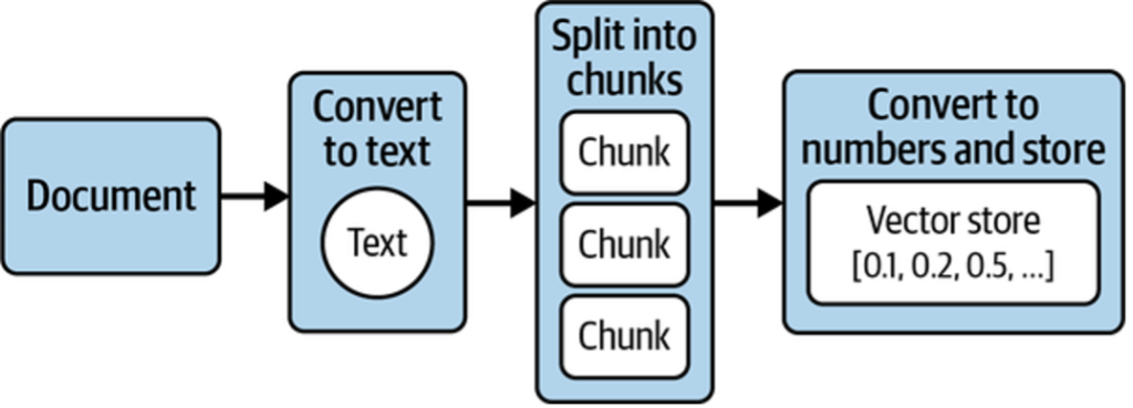
To achieve this, four key steps are required (shown in Figure 1):
- Extract text from the document.
- Split the text into manageable chunks.
- Convert the text into numerical representations.
- Store these representations so relevant sections can be retrieved quickly for a given question.
As illustrated in Figure 1, this workflow—called ingestion—transforms documents into numerical representations that computers can analyze and store efficiently. These representations are called embeddings, and they are stored in a specialized database known as a vector store. Next, we’ll take a closer look at embeddings and why they matter.
Embeddings: Converting Text to Numbers
An embedding represents text as a long sequence of numbers. This representation is lossy—you can’t reconstruct the original text—so systems usually store both the text and its embedding. The benefit is that numbers can be compared mathematically, letting computers work with language in powerful ways.
Embeddings Before LLMs
Embeddings predate LLMs and were widely used for tasks like search and spam detection. A classic example is the bag-of-words model:
- Start with a set of sentences.
- List all unique words across them.
- For each sentence, count how often each word appears.
Table 1 shows the resulting embeddings.
| Word | What a sunny day. | Such bright skies today. | I haven’t seen a sunny day in weeks. |
|---|---|---|---|
| what | 1 | 0 | 0 |
| a | 1 | 0 | 1 |
| sunny | 1 | 0 | 1 |
| day | 1 | 0 | 1 |
| such | 0 | 1 | 0 |
| bright | 0 | 1 | 0 |
| skies | 0 | 1 | 0 |
| today | 0 | 1 | 0 |
| I | 0 | 0 | 1 |
| haven’t | 0 | 0 | 1 |
| seen | 0 | 0 | 1 |
| in | 0 | 0 | 1 |
| weeks | 0 | 0 | 1 |
These vectors are called sparse embeddings because most values are zero. They work well for keyword search and basic classification (such as spam filtering), but they don’t capture meaning. Phrases like “sunny day” and “bright skies” appear unrelated despite their similar semantics, making such systems easy to fool with synonyms.
LLM-Based Embeddings
Modern semantic embeddings solve this by encoding meaning rather than exact words. They evolved from the same training principles as LLMs: learning how words relate to each other based on large text corpora.
An embedding model takes text and outputs a dense numerical vector—typically 100 to 2,000 floating-point values—that represents its semantic meaning. These are called dense embeddings because most dimensions are nonzero.
Different embedding models produce vectors of different sizes and values, and embeddings from different models are not directly comparable.
Semantic Embeddings Explained
Take the words lion, pet, and dog. Intuitively, pet and dog are more similar—but computers don’t have this intuition. To reason about meaning, words must be translated into numbers.
Semantic embeddings do exactly this by mapping words (or sentences) to numerical vectors that capture meaning. As shown in Figure 2, the numbers themselves aren’t meaningful; what matters is that embeddings for similar concepts are closer together than those for unrelated ones.
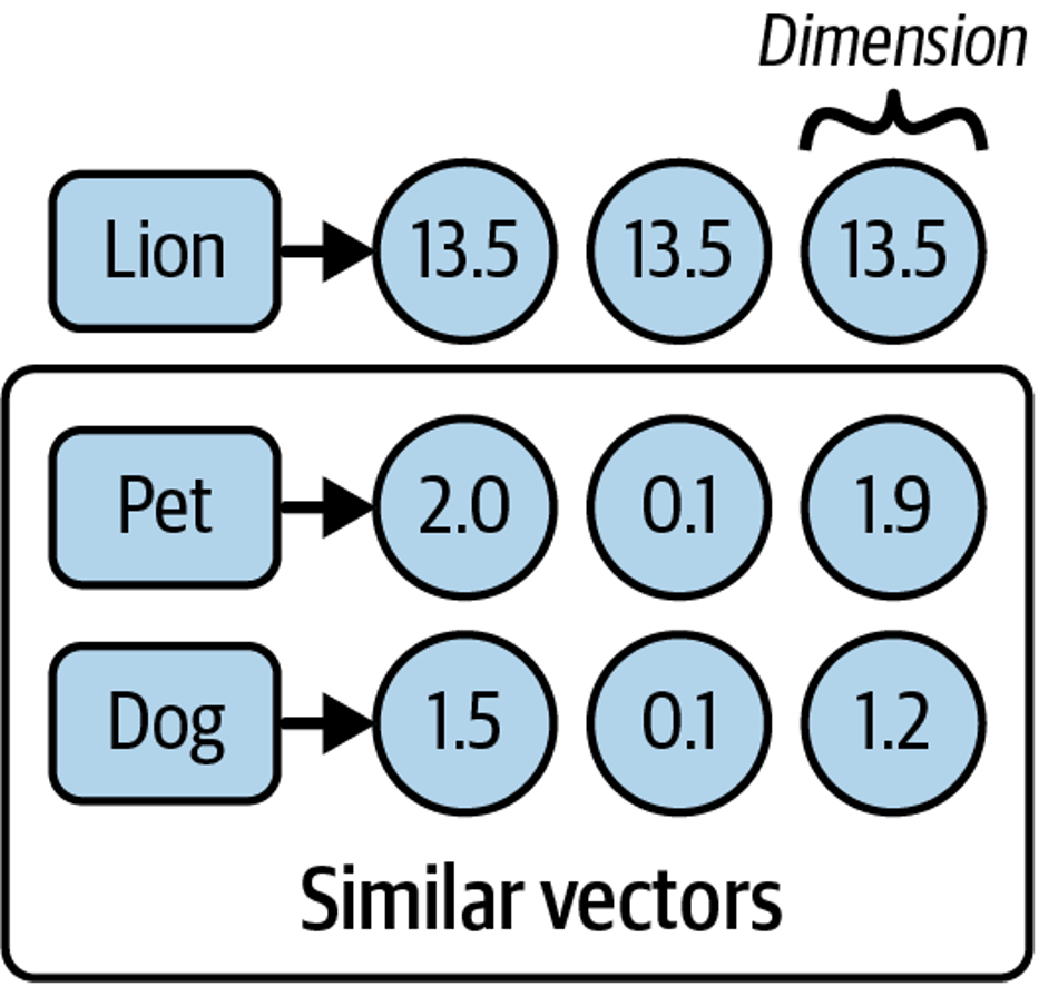
When plotted in a multidimensional space (Figure 3), vectors for pet and dog appear closer than either is to lion. Similarity can be measured by distance or angle between vectors: smaller distances or narrower angles indicate greater semantic similarity.

A common metric for this is cosine similarity, which produces a value between –1 and 1. Higher values indicate more similar meanings—for example, pet and dog might score 0.75, while pet and lion might score 0.1.
This ability to encode meaning numerically and compare it mathematically is what allows LLM-based systems to retrieve the most relevant documents—such as finding the right sections of a large PDF to answer a question.
Other Uses for Embeddings
Embeddings enable a wide range of applications:
- Similarity search: Nearby vectors represent related content.
- Clustering: Groups of close vectors can reveal topics.
- Averaging: Multiple embeddings can be combined to represent larger bodies of text.
- Vector arithmetic: Simple math can capture relationships (for example, king – man + woman ≈ queen).
- Multimodal use: Embeddings can also represent images, audio, and video.
Because of these properties, embeddings are commonly used for search, clustering, classification, recommendations, and anomaly detection—making them a versatile foundation for many LLM-powered systems.
Converting Your Documents into Text
The first preprocessing step is converting documents into text. This requires parsing each source with minimal quality loss. LangChain simplifies this with document loaders, which extract content into a standardized Document object containing text and metadata.
For example, loading a simple .txt file looks like this:
from langchain_community.document_loaders import TextLoader
loader = TextLoader("./test.txt")
loader.load()
The output is a list of Document objects:
[Document(page_content='text content \n', metadata={'line_number': 0, 'source':
'./test.txt'})]
All LangChain document loaders follow the same pattern:
- Choose a loader for your document type.
- Instantiate it with configuration details (such as file path or URL).
- Call
load()to get documents ready for the next stage.
Beyond .txt, LangChain supports formats like CSV, JSON, and Markdown, as well as integrations with tools such as Slack and Notion. It can also load and parse web pages. For example, using WebBaseLoader:
Install the dependency:
pip install beautifulsoup4
from langchain_community.document_loaders import WebBaseLoader
loader = WebBaseLoader("https://www.langchain.com/")
loader.load()
For PDFs, such as Tesla’s annual report, LangChain provides a dedicated loader:
# install the pdf parsing library
# pip install pypdf
from langchain_community.document_loaders import PyPDFLoader
loader = PyPDFLoader("./test.pdf")
pages = loader.load()
At this point, the text is extracted and stored as Document objects—but the result may be very large. Long documents (often 100,000+ characters) exceed the context window limits of most LLMs and embedding models. To address this, the text must be split into smaller chunks that can later be embedded and searched.
LLMs and embedding models have a fixed context window, which limits the combined size of input and output. Context windows are measured in tokens (for example, 8,192 tokens), where each token typically represents three to four characters of English text. This constraint makes chunking a necessary next step.
Splitting Your Text into Chunks
Splitting large documents into chunks sounds simple, but preserving semantic coherence is not. Chunks should stay small enough for LLMs while keeping related text together. LangChain addresses this with RecursiveCharacterTextSplitter, which:
- Uses an ordered list of separators (by default: paragraphs
\n\n, lines\n, then words). - Splits text to respect a target chunk size (for example, 1,000 characters).
- Recursively applies smaller separators if a chunk is still too large.
- Outputs each chunk as a
Document, preserving original metadata and adding position data.
Here’s a basic example:
from langchain_text_splitters import RecursiveCharacterTextSplitter
loader = TextLoader("./test.txt") # or any other loader
docs = loader.load()
splitter = RecursiveCharacterTextSplitter(
chunk_size=1000,
chunk_overlap=200,
)
splitted_docs = splitter.split_documents(docs)
This produces overlapping chunks (200 characters by default) to preserve context across boundaries, split along natural text structure like paragraphs and lines.
Splitting Code and Structured Text
RecursiveCharacterTextSplitter also supports structured formats such as code and Markdown. Language-specific separators ensure logical units—like functions—stay together, often eliminating the need for overlap.
Example with Python code:
from langchain_text_splitters import (
Language,
RecursiveCharacterTextSplitter,
)
PYTHON_CODE =
"""
def hello_world():
print("Hello, World!")
# Call the function
hello_world()
"""
python_splitter = RecursiveCharacterTextSplitter.from_language(
language=Language.PYTHON, chunk_size=50, chunk_overlap=0
)
python_docs = python_splitter.create_documents([PYTHON_CODE])
Output:
[Document(page_content='def hello_world():\n print("Hello, World!")'),
Document(page_content='# Call the function\nhello_world()')]
Here, from_language configures separators for a specific language. The create_documents method is useful when splitting raw strings instead of loader-produced documents.
Passing Metadata
You can also attach metadata when splitting raw text. The metadata list must match the number of input strings.
Markdown example:
markdown_text =
"""
# LangChain
⚡ Building applications with LLMs through composability ⚡
## Quick Install
```bash
pip install langchain
```
As an open source project in a rapidly developing field, we are extremely open
to contributions.
"""
md_splitter = RecursiveCharacterTextSplitter.from_language(
language=Language.MARKDOWN, chunk_size=60, chunk_overlap=0
)
md_docs = md_splitter.create_documents([markdown_text],
[{"source": "https://www.langchain.com"}])Output:
[Document(page_content='# LangChain',
metadata={"source": "https://www.langchain.com"}),
Document(page_content='⚡ Building applications with LLMs through composability
⚡', metadata={"source": "https://www.langchain.com"}),
Document(page_content='## Quick Install\n\n```bash',
metadata={"source": "https://www.langchain.com"}),
Document(page_content='pip install langchain',
metadata={"source": "https://www.langchain.com"}),
Document(page_content='```', metadata={"source": "https://www.langchain.com"}),
Document(page_content='As an open source project in a rapidly developing field,
we', metadata={"source": "https://www.langchain.com"}),
Document(page_content='are extremely open to contributions.',
metadata={"source": "https://www.langchain.com"})]
Two things to note:
- Text is split along natural structural boundaries (headings, code blocks, paragraphs).
- Metadata is preserved on every chunk, making it easy to trace each piece back to its source.
Generating Text Embeddings
LangChain provides an Embeddings interface for working with text embedding models such as OpenAI, Cohere, and Hugging Face. It supports two core operations: embedding multiple documents at once or embedding a single query.
Here’s an example using OpenAI’s embedding model:
from langchain_openai import OpenAIEmbeddings
model = OpenAIEmbeddings()
embeddings = model.embed_documents([
"Hi there!",
"Oh, hello!",
"What's your name?",
"My friends call me World",
"Hello World!"
])
The output is a list of numerical vectors, one per input string. Embedding documents in batches is more efficient than embedding them individually.
Putting everything together, a typical preprocessing pipeline consists of:
- Loading documents and converting them to text
- Splitting large documents into smaller chunks
- Generating embeddings for each chunk
Here’s an end-to-end example:
from langchain_community.document_loaders import TextLoader
from langchain_text_splitters import RecursiveCharacterTextSplitter
from langchain_openai import OpenAIEmbeddings
## Load the document
loader = TextLoader("./test.txt")
doc = loader.load()
"""
[
Document(page_content='Document loaders\n\nUse document loaders to load data
from a source as `Document`\'s. A `Document` is a piece of text\nand
associated metadata. For example, there are document loaders for
loading a simple `.txt` file, for loading the text\ncontents of any web
page, or even for loading a transcript of a YouTube video.\n\nEvery
document loader exposes two methods:\n1. "Load": load documents from
the configured source\n2. "Load and split": load documents from the
configured source and split them using the passed in text
splitter\n\nThey optionally implement:\n\n3. "Lazy load": load
documents into memory lazily\n', metadata={'source': 'test.txt'})
]
"""
## Split the document
text_splitter = RecursiveCharacterTextSplitter(
chunk_size=1000,
chunk_overlap=20,
)
chunks = text_splitter.split_documents(doc)
## Generate embeddings
embeddings_model = OpenAIEmbeddings()
embeddings = embeddings_model.embed_documents(
[chunk.page_content for chunk in chunks]
)
"""
[[0.0053587136790156364,
-0.0004999046213924885,
0.038883671164512634,
-0.003001077566295862,
-0.00900818221271038, ...], ...]
"""
Once embeddings are generated, they are ready to be stored in a vector store for efficient similarity search and retrieval.
Storing Embeddings in a Vector Store
To compare embeddings efficiently, you need a vector store—a database optimized for storing vectors and performing similarity calculations such as cosine similarity. Unlike traditional databases designed for structured data, vector stores handle unstructured data (text, images) while still supporting CRUD and search operations.
Vector stores enable scalable AI applications, such as question answering over large document collections (shown in Figure 4).

When a query is issued, its embedding is computed and compared against stored embeddings to retrieve the most similar documents.
There are many vector store providers, each with different trade-offs around performance, cost, scalability, metadata filtering, and multitenancy. However, vector stores also introduce challenges: they are relatively new, can be complex to manage, and add operational overhead.
To reduce this complexity, vector search can be added directly to PostgreSQL using the pgvector extension. This allows you to use a familiar relational database for both transactional data and vector search.
Getting Set Up with PGVector
To use PostgreSQL with pgvector:
- Install Docker.
- Run the following command to start Postgres with pgvector on port 6024:
docker run \
--name pgvector-container \
-e POSTGRES_USER=langchain \
-e POSTGRES_PASSWORD=langchain \
-e POSTGRES_DB=langchain \
-p 6024:5432 \
-d pgvector/pgvector:pg16
- Save the connection string for later use:
postgresql+psycopg://langchain:langchain@localhost:6024/langchain
Working with Vector Stores
Building on the previous steps (loading, splitting, and embedding), here’s how to store document embeddings in PGVector:
# first, pip install langchain-postgres
from langchain_community.document_loaders import TextLoader
from langchain_openai import OpenAIEmbeddings
from langchain_text_splitters import RecursiveCharacterTextSplitter
from langchain_postgres.vectorstores import PGVector
from langchain_core.documents import Document
import uuid

# Load the document, split it into chunks
raw_documents = TextLoader('./test.txt').load()
text_splitter = RecursiveCharacterTextSplitter(chunk_size=1000,
chunk_overlap=200)
documents = text_splitter.split_documents(raw_documents)

# embed each chunk and insert it into the vector store
embeddings_model = OpenAIEmbeddings()
connection = 'postgresql+psycopg://langchain:langchain@localhost:6024/langchain'
db = PGVector.from_documents(documents, embeddings_model, connection=connection)
This step:
- Connects to Postgres
- Creates required tables (if needed)
- Generates embeddings
- Stores embeddings, text, and metadata
Searching the Vector Store
db.similarity_search("query", k=4)
This process embeds the query, finds the most similar stored vectors, and returns the corresponding Document objects ranked by relevance.
Adding and Deleting Documents
You can insert additional documents into an existing vector store:
ids = [str(uuid.uuid4()), str(uuid.uuid4())]
db.add_documents(
[
Document(
page_content="there are cats in the pond",
metadata={"location": "pond", "topic": "animals"},
),
Document(
page_content="ducks are also found in the pond",
metadata={"location": "pond", "topic": "animals"},
),
],
ids=ids,
)
Documents can later be removed using their IDs:
db.delete(ids=[1])
Using explicit IDs allows documents to be updated or deleted as your data evolves.
Tracking Changes to Your Documents
A major challenge with vector stores is handling frequently changing data. Any change can require re-indexing, which may trigger expensive embedding recomputation and duplicate content. LangChain addresses this with an indexing API that keeps your documents synchronized with the vector store.
This API uses a RecordManager to track document writes. For each document, it stores:
- A hash of the document content and metadata
- The write timestamp
- A source ID identifying the original data source
This allows LangChain to detect changes and avoid unnecessary re-indexing.
Cleanup Modes
The indexing API supports different cleanup strategies:
- None: No automatic cleanup; you manage old data manually.
- Incremental: Replaces prior versions when a document’s content changes.
- Full: Additionally removes any documents not included in the current indexing run.
These modes help handle updates, processing changes, or deleted source documents.
Example: Using the Indexing API with PGVector
Below is an example using PostgreSQL as both the vector store and the record manager:
from langchain.indexes import SQLRecordManager, index
from langchain_postgres.vectorstores import PGVector
from langchain_openai import OpenAIEmbeddings
from langchain.docstore.document import Document

connection = "postgresql+psycopg://langchain:langchain@localhost:6024/langchain"
collection_name = "my_docs"
embeddings_model = OpenAIEmbeddings(model="text-embedding-3-small")
namespace = "my_docs_namespace"

vectorstore = PGVector(
embeddings=embeddings_model,
collection_name=collection_name,
connection=connection,
use_jsonb=True,
)

record_manager = SQLRecordManager(
namespace,
db_url="postgresql+psycopg://langchain:langchain@localhost:6024/langchain",
)

# Create the schema if it doesn't exist
record_manager.create_schema()

# Create documents
docs = [
Document(page_content='there are cats in the pond', metadata={
"id": 1, "source": "cats.txt"}),
Document(page_content='ducks are also found in the pond', metadata={
"id": 2, "source": "ducks.txt"}),
]

# Index the documents
index_1 = index(
docs,
record_manager,
vectorstore,
cleanup="incremental",  # prevent duplicate documents
source_id_key="source", # use the source field as the source_id
)
print("Index attempt 1:", index_1)

# Second indexing skips unchanged documents
index_2 = index(
docs,
record_manager,
vectorstore,
cleanup="incremental",
source_id_key="source",
)
print("Index attempt 2:", index_2)

# Modify a document; old versions from the same source are replaced
docs[0].page_content = "I just modified this document!"
index_3 = index(
docs,
record_manager,
vectorstore,
cleanup="incremental",
source_id_key="source",
)
print("Index attempt 3:", index_3)
In this workflow, the record manager tracks what has already been indexed, and the index function keeps the vector store in sync. Using incremental cleanup ensures updated documents replace older versions without duplicating content.
Indexing Optimization
Basic RAG indexing—splitting text into chunks and embedding them—can lead to inconsistent retrieval and more hallucinations, especially when documents include tables or images. Optimized indexing strategies improve accuracy and performance. Three approaches are commonly used: MultiVectorRetriever, RAPTOR, and ColBERT. Here, we focus on MultiVectorRetriever.
MultiVectorRetriever
Documents containing a mix of text and tables cannot be embedded by naive text splitting alone, because important information (like tables) may be lost. MultiVectorRetriever decouples retrieval context from answer synthesis content:
- Generate embeddings for summaries of tables or complex sections.
- Store full tables or original content in a separate document store.
- When a query retrieves a summary, fetch the full original content to provide complete context to the LLM.
This approach ensures the LLM has all relevant information while keeping retrieval efficient.
Example: Summarizing and Indexing Documents
from langchain_community.document_loaders import TextLoader
from langchain_text_splitters import RecursiveCharacterTextSplitter
from langchain_openai import OpenAIEmbeddings, ChatOpenAI
from langchain.retrievers.multi_vector import MultiVectorRetriever
from langchain.storage import InMemoryStore
from langchain_core.documents import Document
import uuid

connection = "postgresql+psycopg://langchain:langchain@localhost:6024/langchain"
collection_name = "summaries"
embeddings_model = OpenAIEmbeddings()

# Load and split document
loader = TextLoader("./test.txt", encoding="utf-8")
docs = loader.load()
splitter = RecursiveCharacterTextSplitter(chunk_size=1000, chunk_overlap=200)
chunks = splitter.split_documents(docs)

# Summarize chunks with an LLM
prompt_text = "Summarize the following document:\n\n{doc}"
llm = ChatOpenAI(temperature=0, model="gpt-3.5-turbo")
summarize_chain = {"doc": lambda x: x.page_content} | prompt_text | llm
summaries = summarize_chain.batch(chunks, {"max_concurrency": 5})

# Set up vector store for summaries and docstore for originals
vectorstore = PGVector(embeddings=embeddings_model,
                       collection_name=collection_name,
                       connection=connection,
                       use_jsonb=True)
store = InMemoryStore()
id_key = "doc_id"
retriever = MultiVectorRetriever(vectorstore=vectorstore, docstore=store, id_key=id_key)

# Link summaries to original documents
doc_ids = [str(uuid.uuid4()) for _ in chunks]
summary_docs = [Document(page_content=s, metadata={id_key: doc_ids[i]})
                for i, s in enumerate(summaries)]

# Add summaries to vector store and original chunks to docstore
retriever.vectorstore.add_documents(summary_docs)
retriever.docstore.mset(list(zip(doc_ids, chunks)))

# Retrieve full context documents based on query
retrieved_docs = retriever.invoke("chapter on philosophy")
Workflow:
- Split document into manageable chunks.
- Summarize chunks with an LLM.
- Store summaries in a vector store for similarity search.
- Store original chunks in a docstore linked to summaries.
- Retrieval first searches summaries, then fetches full original content for context.
This ensures high fidelity in responses, even with mixed-content documents like tables, images, or code.
RAPTOR and ColBERT: Advanced Indexing Optimizations
When working with RAG systems, a naive k-nearest neighbors (k-NN) retrieval over chunks can struggle to handle:
- Lower-level questions that reference specific facts in a single document.
- Higher-level questions that require synthesizing ideas across many documents.
To address this, two advanced strategies are commonly used: RAPTOR and ColBERT.
RAPTOR: Recursive Abstractive Processing for Tree-Organized Retrieval
RAPTOR is designed to handle both granular and high-level questions by recursively summarizing documents in a tree-like structure:
- Summarize individual documents to capture core concepts.
- Embed and cluster these summaries to group related ideas.
- Summarize each cluster to produce higher-level concepts.
- Repeat recursively to create a tree of summaries, from low-level details to high-level abstractions.
- Index both summaries and original documents, ensuring coverage for queries at any level.
This approach allows the retrieval system to answer both specific and broad questions efficiently.
Visual idea:
Document chunks -> Summaries -> Cluster summaries -> Recursive higher-level summaries
ColBERT: Optimizing Embeddings
Standard embedding models compress an entire document into a fixed-length vector. While this captures semantic meaning, it may include irrelevant or redundant information, leading to hallucinations when used by LLMs.
ColBERT solves this by generating contextual embeddings for each token and performing fine-grained similarity scoring:
- Compute embeddings for every token in both the query and the document.
- Calculate similarity between each query token and all document tokens.
- Aggregate the maximum similarity scores for each query token to score the document.
This token-level late interaction ensures more precise retrieval and reduces noise from irrelevant content.
Example: Using ColBERT with RAGatouille
# Install RAGatouille (ColBERT interface)
# !pip install -U ragatouille
from ragatouille import RAGPretrainedModel
import requests

# Load pre-trained ColBERT model
RAG = RAGPretrainedModel.from_pretrained("colbert-ir/colbertv2.0")

# Function to get Wikipedia page content
def get_wikipedia_page(title: str) -> str:
    URL = "https://en.wikipedia.org/w/api.php"
    params = {
        "action": "query",
        "format": "json",
        "titles": title,
        "prop": "extracts",
        "explaintext": True,
    }
    headers = {"User-Agent": "RAGatouille_tutorial/0.0.1"}
    response = requests.get(URL, params=params, headers=headers)
    page = next(iter(response.json()["query"]["pages"].values()))
    return page.get("extract")

# Retrieve and index the page
full_document = get_wikipedia_page("Hayao_Miyazaki")
RAG.index(collection=[full_document],
          index_name="Miyazaki-123",
          max_document_length=180,
          split_documents=True)

# Search example
results = RAG.search(query="What animation studio did Miyazaki found?", k=3)

# Use as LangChain retriever
retriever = RAG.as_langchain_retriever(k=3)
retriever.invoke("What animation studio did Miyazaki found?")
Benefits of RAPTOR + ColBERT:
- RAPTOR: Handles queries at multiple abstraction levels.
- ColBERT: Provides precise token-level similarity for better retrieval.
- Combined: Produces highly relevant document chunks for LLM context, reducing hallucinations.
This is especially valuable for long, complex documents or collections with mixed content types (text, tables, etc.).
Summary
In this chapter, you learned how to prepare and preprocess documents for LLM applications using LangChain. Document loaders allow you to extract text from a variety of sources, including .txt files, PDFs, web pages, and platforms like Slack or Notion. Once the text is extracted, text splitters, such as RecursiveCharacterTextSplitter, break large documents into semantically meaningful chunks that retain context and fit within the model’s context window. These chunks are then converted into numeric embeddings using models like OpenAI’s, which capture the semantic meaning of the text. Cosine similarity and other metrics can be used to compare these embeddings and find related chunks efficiently.
Vector stores, like PGVector, provide a way to store these embeddings and support CRUD operations along with fast similarity searches. Using the indexing API and record managers, you can track changes in your documents, avoid duplication, and selectively re-index only updated content. Indexing optimization strategies further improve retrieval quality and relevance: MultiVectorRetriever handles documents with mixed content, like tables, by linking summaries to full content; RAPTOR recursively summarizes documents into a hierarchical tree of concepts for both fact-based and high-level queries; and ColBERT produces token-level embeddings to enhance precision and reduce irrelevant retrievals.
By combining document loaders, splitters, embeddings, vector stores, and optimized indexing strategies, you create a robust pipeline for semantic search and retrieval. This ensures that your AI application can efficiently locate the most relevant information and provide accurate, context-aware answers. Chapter 3 will build on this foundation by showing how to retrieve these relevant chunks from the vector store and feed them into an LLM for high-quality output.